Paper URL: https://arxiv.org/pdf/2502.06501
Code URL: https://github.com/quhongyu/ClusPro

Conference: ICLR’25

🚧 UNDER CONSTRUCTION 🚧

Paper URL: https://openaccess.thecvf.com/content/CVPR2025/papers/Sun_Unsupervised_Continual_Domain_Shift_Learning_with_Multi-Prototype_Modeling_CVPR_2025_paper.pdf
Code URL: TBD

Conference: CVPR’25

TL;DR

To overcome the adaptivity gap issue in Unsupervised Continual Domain Shift Learning, the paper proposes Multi-Prototype Modeling (MPM) , a method comprises two main parts: Multi-Prototype Learning (MPL) and Bi-Level Graph Enhancer (BiGE).

Introduction

What is Unsupervised Continual Domain Shift Learning (UCDSL)?

Unsupervised Continual Domain Shift Learning (UCDSL) aims to adapt a pre-trained model to dynamically shifting target domains without access to labeled data from either the source or target domains.

Existing Methods of UCDSL

Existing methods attempt to learn a universal classifier for all domains by enforcing feature alignment across different domains. ==However, this assumption is not guaranteed and the classifier may deviate significantly from the optimal classifier for a specific target domain.==

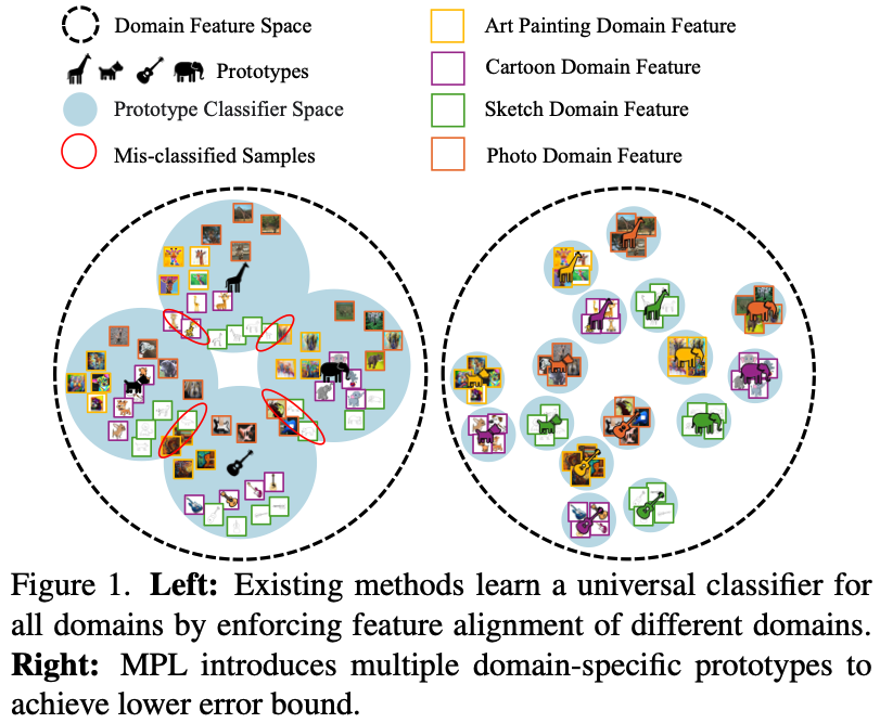
As shown in the left image, existing methods pursue the alignment of the same classes across all domains. This leads to the deviation from the optimal classifier for each domain, causing mis-classification.

Motivation

To address this issue, the paper ==introduces multiple domain-specific prototypes to enrich the hypothesis space and achieve more comprehensive representations==, as shown in the right image.

This brings the following benefits:

1. MPL enriches the hypothesis space by introducing multiple harmoniously composited domain-specific prototypes, leading to improved generalization for unseen domains.
2. MPL preserves complementary information from multiple domains to reduce the adaptivity gap, resulting in enhanced domain adaptation ability.
3. During adaptation, MPL explicitly preserves knowledge from previously encountered domains by retaining the corresponding prototypes.

To enhance the feature representations, Bi-Level Graph Enhancer is introduced as well. It leverages complementary information from two orthogonal perspectives: domain-wise and category-wise.

Paper URL: https://arxiv.org/pdf/2503.01776
Code URL: https://github.com/neilwen987/CSR_Adaptive_Rep

Conference: ICML’25 Oral

TL;DR

This paper introduces CSR, an effective learning method for sparse adaptive representations. It combines a task-specific sparse contrastive learning loss with a reconstructive loss to maintain overall embedding quality.

Intro

MRL, as an existing method to compress representations, truncates the linear layers into a set of target sizes to reflect representations of various dimensions.

However, MRL faces two key constraints:

1. it requires (full) training of the backbone parameters;
2. its performance often deteriorates a lot under small hidden dimensions.

   Method

   CSR combines sparse contrastive learning and sparse autoencoding to maintain overall embedding quality.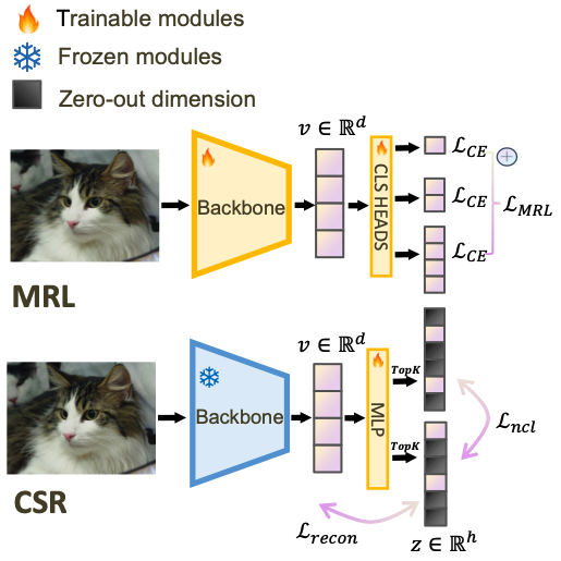
   

   Sparse Autoencoders(SAEs)

   SAEs aim to extract a sparse representation $z_k$ by learning to reconstruct the dense feature from $z_k$.

Denote the (weights, bias) of encoder and decoder as $(W_{enc},b_{enc})$ and $(W_{dec},b_{pre})$. And $f(x)$ represents the dense feature of input $x$.

Encoding

$$z_k:=\sigma^+(\text{TopK}(W_{enc}(f(x)-b_{pre})+b_{enc}))$$

$\text{TopK}$ gets $K$ largest values. $\sigma^+(\cdot)=max(0,\cdot)$ is the ReLU activation.
This process encodes the dense representations into sparse representations, with only $K$ non-zero values.

Decoding

$$\widehat{f(x)_k}:=W_{dec}z_k+b_{pre}$$

This process decodes and reconstructs the original embedding using sparse representation $z_k$. To make $\widehat{f(x)_k}$ as similar to $f(x)$ as possible, it uses L2 reconstruction loss as the main training objective:

$$\mathcal{L}(k)=||f(x) - \widehat{f(x)_k}||_2^2.$$

Dead Latents

As the large number of zeros in sparse representations, a lot of latent dimensions remain inactive during training - a phenomenon called the Dead Latents. This is one of the reasons of the performance degradation.
To mitigate this issue, an auxiliary loss $\mathcal{L}_{aux}$ and Multi-TopK losses are proposed.

Auxiliary Loss

$$\mathcal{L}_{aux} = ||e-\hat{e}||_2^2,$$

where $e=f(x)-\widehat{f(x)}$, and $\hat{e}=W_{dec}z$. This is the forced reconstruction using the top-$k_{aux}$ dead latents.

Multi-TopK Losses

An extra $4k$ reconstruction is added.

The overall construction loss is

$$\mathcal{L}_{recon}=\mathcal{L}(k)+\frac{1}{8}\mathcal{L}(4k)+\beta\mathcal{L}_{aux}.$$

Sparse Contrastive Learning

Simply reconstruction is not enough to make sparse representations distinguishable. So contrastive learning is introduced to enhance the semantic discriminative power of sparse representations.

Supposing batch size $\mathcal{B}$. $z_i$ represents the $i$-th sample in the batch. The contrastive loss is defined as

$$\mathcal{L}_{cl}=-\frac{1}{\mathcal{B}}\sum^{\mathcal{B}}_{i=1}\log{\frac{\exp(z_i^Tz_i)}{\exp(z_i^Tz_i)+\sum_{j\ne i}^{\mathcal{B}}\exp(z_i^Tz_j)}}$$

This makes each latent representations closer to the positive samples (itself) and further to the negative samples (other representations).
Notice that all the $z$ are non-negative by $\text{ReLU} + \text{TopK}$ selection, thus this contrastive loss is a variant of the Non-negative Contrastive Loss (NCL).

Theorem 5. Under mild conditions, the solution $\phi(x)$ is the unique solution to the NCL objective. As a result, NCL features are identifiable and disentangled.

According to the above theorem, the sparse contrastive loss tends to relate each latent dimension to a specific stable and distinguishable semantic factor. It also helps mitigate the dead latents issue.

Overall Training Objectiveness

$$\mathcal{L}_{CSR}=\mathcal{L}_{recon}+\gamma\mathcal{L}_{ncl}.$$

Paper URL: https://arxiv.org/pdf/2501.09446
Code URL: https://doublevisualdefense.github.io/

TL;DR

This paper aims to enhance the robustness of vision-language models against adversarial visual perturbations. It proposes Double Visual Defense, a large-scale adversarial vision-language pre-training method. This method contains two stages: Adversarial Contrastive Pre-Training and Adversarial Visual Instruction-Tuning. In experiments, it showcases robustness improvement, stronger zero-shot recognition capability, fewer hallucinations and superior reasoning performance.

Intro

Traditional adversarial robustness methods focus more on post-hoc fine-tuning. Double Visual Defense, in contrast, propose to both CLIP pre-training and visual instruction tuning.

Method

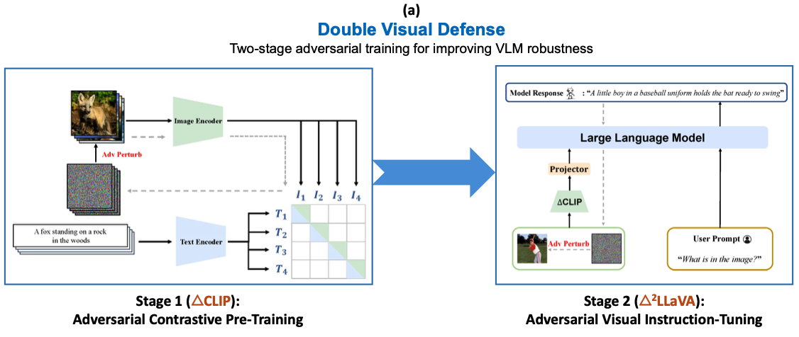
Adversarial Contrastive Pre-Training

∆CLIP is trained to predict the right image-text pairings given adversarial images that are optimized to fool the model into predicting incorrect image-text pairings.

Adversarial Visual Instruction-Tuning

Q&A

1. Is adversarial robustness the same thing as domain robust? I’ve done research on test-time prompt tuning to enhance zero-shot and cross-domain generalization of vision-language models. Are they the same? If not, what‘s the difference between cross-domain, out-of-distribution and adversarial robustness?

Original: https://zhuanlan.zhihu.com/p/102870562

What is OOD Detection?

OOD(out-of-distribution) detection aims to detect an OOD sample, which is the opposite of ID(in-distribution) sample.

In traditional machine learning methods, the training and test data are assumed to be independent identical distribution(IID). However, in real-world scenario, test samples are likely to be OOD, or outlier. Traditional deep learning models often consider an OOD sample as a class of ID samples with high confidence, which is not reasonable. Thus it is meaningful for models to recognize OOD samples, especially for AI security areas.

Methods

Existing OOD Detection methods can be roughly divided into 4 categories:

• Softmax-based methods.
• Uncertainty methods.
• Generative model methods.
• Classifier methods.

  Softmax-based Methods

  Softmax-based methods get the softmax values of the outputs of a pre-trained model. And find out how OOD and ID samples distribute by statistical analysis. It aims to enlarge the difference between OOD and ID distributions.

Softmax-based methods are simple, entirely training-free yet effective, without the need to change model structure.

SMOOD

Paper URL: https://arxiv.org/abs/1610.02136

SMOOD(SoftMax OOD) is the very first work of OOD Detection task. It proposes an OOD baseline method. Its main insights are:

1. Correctly classified examples tend to have greater maximum softmax probabilities than erroneously classified and out-of-distribution examples, allowing for their detection.
2. Proposed a simple yet effective baseline method to detect whether a sample is mis-classified or out-of-distribution.

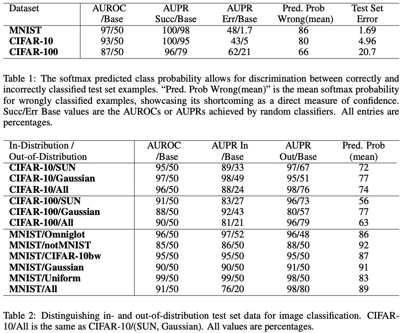
The above tables show that using simply max softmax probabilities to in- or out-of-distribution samples is effective. But it can not tell if the model wrongly classifies the sample.

In conclusion, SMOOD justifies the softmax output of the model differs when an in- or out-of-distribution sample is given. So they can be effectively discriminated by choosing a proper threshold.

ODIN

Paper URL: https://arxiv.org/abs/1706.02690

SMOOD is simple and effective. But the effect is not good enough. To achieve better results, ODIN proposes to enlarge the gap between in- and out-of-distribution softmax probabilities.

Based on above thoughts, it introduces two main methods:

• Temperature Scaling
• Input Preprocessing

Temperature Scaling

$$p_i(x;T)=\frac{\exp(f_i(x)/T)}{\sum_{j=1}^N\exp(f_i(x)/T)}$$

A $T$ that is large enough makes the softmax probabilities close enough to $\frac{1}{N}$.

Image Preprocessing

ODIN preprocesss the input by adding small perturbations:

$$\widetilde{x}=x-\epsilon\text{sign}(-\bigtriangledown_x\log(p_{\hat{y}}(x;T))$$

$x$ and $\epsilon$ denote the input sample and perturbation magnitude, respectively.
In adversarial examples(where $\widetilde{x}=x+\epsilon\text{sign}$), small perturbations are added to decrease the softmax score for the true label and force the model to make a wrong prediction. In ODIN, the goal is the opposite: it aims to increase the softmax score of any given input.
Why it works? ID sample confidence are increased dramatically while OOD sample confidence stays the same. Thus the confidence gap between ID and OOD samples is enlarged.

Uncertainty Methods

Uncertainty-based methods mainly learns the uncertainty of the model predictions. The uncertainty should be high given an OOD sample and low given an ID sample.

Learning Confidence for OOD Detection

Paper URL: https://arxiv.org/abs/1802.04865

Motivation. In this paper the authors propose an idea that a network can estimate its prediction confidence and ask for “hints”.

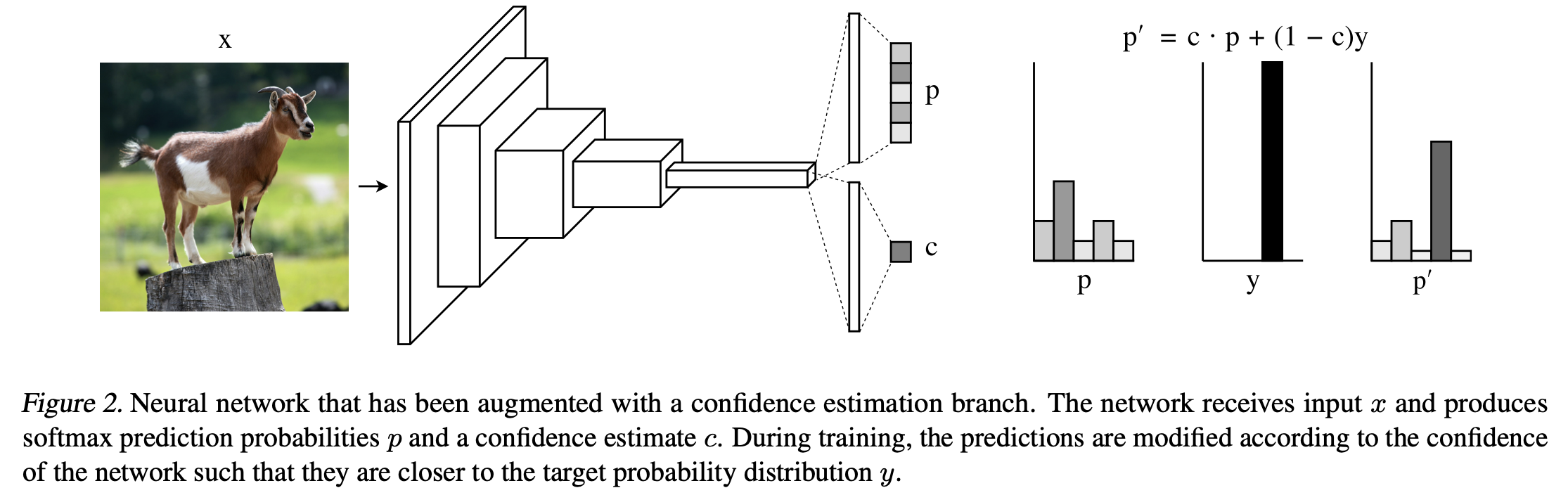
In order to estimate the confidence of the prediction, a confidence estimation branch is added in parallel with the original class prediction branch, as shown in the above figure. It receives the same input as the class prediction branch and outputs the confidence.
The confidence branch contains one or more fully-connected layers, with the final layer outputting a single scalar $c$ between 0 and 1 (parameterized as a sigmoid).
The output of the prediction and confidence branch would be

$$p, c = f(x, \Theta), p_i,c\in[0,1],\sum_{i=1}^Mp_i=1.$$

To “hint” the model, the softmax prediction probabilities are adjusted by interpolating between the original predictions $p$ and the target probability distribution $y$ during training, where the degree of interpolation is indicated by the network’s confidence $c$:

$$p_i' = c \cdot p_i + (1-c)y_i.$$

The loss function $\mathcal{L}_t$ should be as usual, except for that the prediction $p$ should be the modified prediction $p’$.

However, if the model always predict the confidence as $0$, the loss will always be the lowest. To prevent this, the confidence loss, a penalty is added to the loss function. This can be interpreted as a binary cross-entropy loss, where the target value is always 1 (i.e., we want the network to always be very confident):

$$\mathcal{L}_c=-\log(c).$$

So the final loss should be:

$$\mathcal{L} = \mathcal{L}_t + \lambda \cdot \mathcal{L}_c,$$

where $\lambda$ is a super parameter.

Multiple Semantic Label Representations

Paper URL: https://arxiv.org/abs/1808.06664